Although we’ve heuristically discussed how it is that neural networks learn and make decisions,
it’s important to actually be able to understand what’s happening on the inside.
This is the field of mechanistic interpretability. If you’d like to explore this more beyond
what is in this chapter, I recommend reading this article by Neel Nanda of Google DeepMind. However, you may need a bit more background than what we’ve
covered in this course before being able to digest some of the topics.
Neural Networks are Function Approximators
One way you can think of neural networks is as universal function approximators. This is a real
mathematical result known as the Universal Approximation Theorem: given a large enough neural
network (layers and layer size), we can theoretically approximate any function to whatever accuracy
we want. Why is this powerful? Because functions describe the world.
One caveat worth keeping in mind: the theorem only guarantees that a good-enough network
exists. It says nothing about whether gradient descent will actually find it, or how big the
neural network needs to be.
This is much more apparent with our point classifier. In the widgets for the point classifier, there was an underlying
function that determined the color of a point.
The point classifier we had did pretty well at approximating this function. It took points on a Cartesian plane, x and y, and predicted whether a point was red or blue.
The digit classifier you’ve developed does something similar. It learns a highly complex function that takes an
image (e.g., a 784-dimensional vector of pixel values) and outputs a prediction of which digit (0 through 9) the image
represents. That answer is understandably unsatisfying.
What does each layer do, and why does any neuron fire? This simple question of what a neural network actually learns
during training goes extremely deep and turns out to be incredibly challenging to answer.
What Neural Networks Learn
Thankfully, the MNIST dataset we’ve been using has been studied extensively, and they’ve found a couple of things.
The initial layers of a neural network tend to learn basic features from the pixel dataset, such as edges, corners,
or simple curves that appear at various places inside the network. In subsequent layers, the neural network combines
these shapes to form more complex patterns such as loops (common in ‘0’, ‘6’, ‘8’, ‘9’). Finally, the network takes
all of the high-level features and uses them to classify the digits properly.
Let’s take a deeper look at what our MNIST digit classifier has learned. Keep in mind that since we randomize the
weights on initialization and have some noise introduced by stochastic gradient descent, different neural networks
learn to recognize digits in different ways.
For this exploration, we’re going to be working with a feedforward neural network with 784 input neurons, 10 output
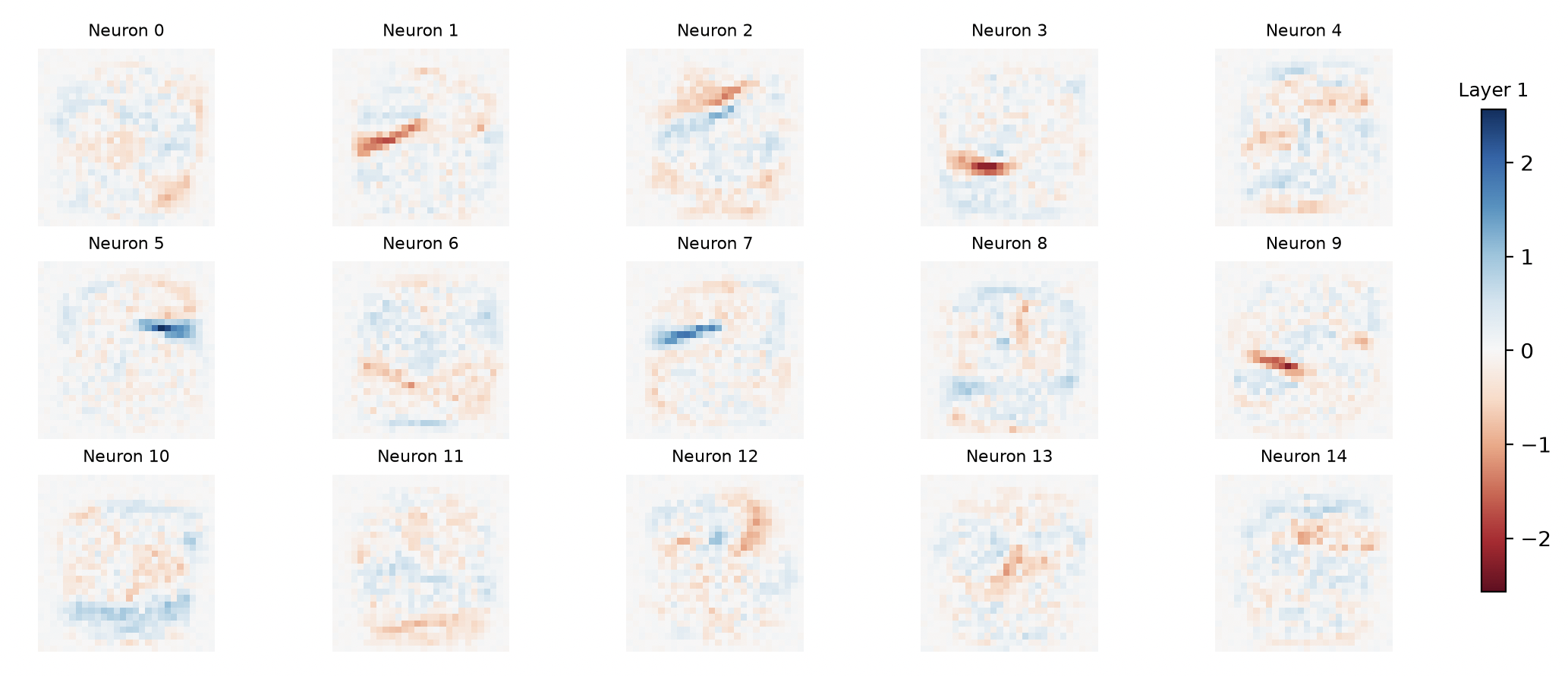
neurons, and 2 hidden layers containing 15 neurons trained on the MNIST digit database. We can visualize what’s going
on between the input layer and first hidden layer by plotting the weights associated with the input layer and each
individual hidden neuron. You can see this in the image below. Red means the weights are pushing the neuron to turn
off, and blue means it’s being pushed to turn on.
The job of the first layer is to take the information from the input and compress it down into
higher order features about the image. Despite being able to see some “obvious” patterns in the
image weights, it’s hard to definitively say what the role of any neuron is. Neurons 5 and 7 look
like they activate for edges detected in the top-right and top-left part of the image respectively,
but it’s possible that they activate for reasons other than edge-detection. The phenomenon where
a neuron activates for different and unrelated concepts rather than just one is known as polysemanticity.
Why would a network learn to do this? The leading explanation is the superposition hypothesis.
The real world contains more distinct features than a network has neurons. Our hidden layers have
15 neurons each, but there are many more strokes, curves, and patterns worth detecting than that.
To squeeze everything in, the network represents features as overlapping combinations spread across
many neurons. This allows more features to get baked into the network than it has dimensions. The
trade-off is that individual neurons end up responding to unrelated features. This in turn makes
them harder to interpret, especially without accounting for how other neurons interact with each
other.
This phenomenon was studied in depth in a 2022 paper, Toy Models of Superposition,
by Nelson Elhage and colleagues at Anthropic. They showed that superposition can actually be
loss-minimizing. The network gains representational capacity at the cost of our ability to
understand it.
Building Up to a Prediction
So the first hidden layer turns raw pixels into a set of simple features. What do the later layers
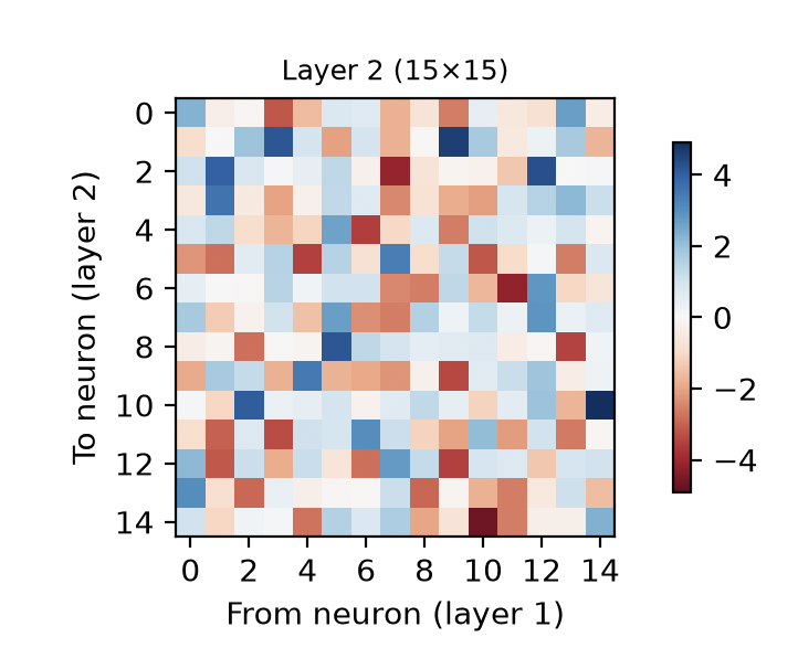
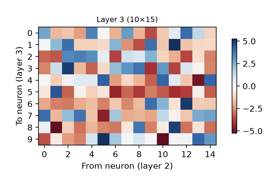
do with them? Let’s look at the weights connecting the two hidden layers, and the weights connecting
the second hidden layer to the output.
We’re going to represent how each layer feeds forward into the next as a heatmap. Each row is a
neuron in the later layer, and each column is a neuron from the layer before it. A blue cell tells
a neuron to activate when an earlier feature is present, and a red cell means to deactivate when it’s
present.
Notice that the second hidden layer never sees a pixel. Its entire view of the world is the 15
activations coming out of the first layer. There are two takeaways from this. First is that there
is some information loss happening at each layer. Second, later layers tend to encode for more
and more abstract features. The neurons combine features learned earlier into more abstract ones.
A loop detector, for instance, might be a neuron with strong positive
weights on a “curve at the top” neuron and a “curve at the bottom” neuron, so it only fires when
both are active at once. This is the composition step from earlier: edges combine into shapes,
and shapes will combine into digits.
You’ve probably also noticed that these weight matrices look like noise. With the first layer, we
could reshape the weights into a 28×28 image and squint at it, because those weights live in pixel
space. The later layers’ weights live in the network’s own internal feature space, and thanks to
superposition, the features themselves are smeared across many neurons. There’s no picture to
reshape them into. This is exactly why interpretability is so hard, and why there’s an entire field, mechanistic interpretability, dedicated to it.
The output layer is where everything finally gets put together. Each of its 10 rows corresponds to
a single digit, and each digit’s neuron acts like an evidence tally: strong positive weights pull in
features consistent with that digit, while negative weights let features vote against it. An “8”
wants the loop detectors on, and a “1” wants them firmly off. Whichever neuron accumulates the most
evidence becomes the network’s prediction.
Looking Forward
There is a lot more to understanding what goes on inside of a neural network, and you could write
a full course on the subject of mechanistic interpretability. However, this is a good starting
point for understanding what neural networks are actually learning when we train them.
In the next chapter, we’re going to review the key ideas behind what we’ve learned in this course,
and what you should continue to do as you dive into the world of machine learning.