Chapter 1: The Structure of Neural Networks

The Difficulty of Image Recognition

When first learning to code, you’re taught to break down programs into smaller, more manageable parts that you can code up. Then, after coding up each tiny piece, you can put them together in order to get a program that does what you originally intended.

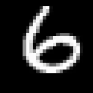
However, there are some problems where this isn’t possible. Image recognition is a classic example. It seems simple because our brains do it automatically, but we take for granted how easily we can recognize the following numbers as 9 and 6:

Actually writing a program that reads handwritten digits would be monstrously difficult. The problem is that handwriting is messy: a digit can vary significantly in size, slant, stroke thickness, and shape. Any fixed set of rules we hard-code would have tons of exceptions. Despite this, people can identify these digits effortlessly, even though they’d struggle to explain exactly how they do it. Without being able to clearly define the process, we can’t write a traditional step-by-step program to solve it.

Because of this, researchers turned to another source for inspiration: the human brain. While we can’t actually emulate the human brain yet, we can use it as a loose analogy to create something similar. In practice, this gives us extremely promising results.

Artificial Neurons

Biological neurons, the building blocks of the brain, are incredibly complex. We can design much simpler artificial neurons that loosely mimic their behavior. Throughout this course, we’ll simply refer to artificial neurons as neurons.

Neurons take in multiple inputs that help them decide whether or not they should fire. Each input then gets multiplied by a weight that signifies its influence. These inputs get summed together into a single value. If it exceeds some cutoff value—called the threshold—the neuron fires and outputs a one. Otherwise, it’ll output a zero. We can describe a neuron algebraically as follows:

The variable $a_j$ is the j-th input to the neuron, and $w_j$ is the corresponding weight. The summation, $\sum\limits_j w_j a_j$, is typically written as the dot product between the inputs and weights, $\overrightarrow w \cdot \overrightarrow a$.

The artificial neuron we’ve described is known as the Perceptron. It’s outdated, but it provides us a good starting point for understanding neurons and neural networks.

Understanding Neurons

A good heuristic for understanding neurons is that they give an answer (output)—yes (one) or no (zero)—based on the answers to previous questions (inputs). Some answers are important (higher weights), and some are useless (near-zero weights). Answers can make it more likely to get a yes (positive weights), while others make it more likely to get a no (negative weights).

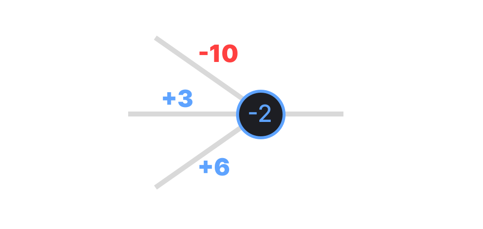
A helpful, although unrealistic, example is deciding whether or not someone—let’s call her Jane—would hang out with her friends. The neuron below represents how Jane might decide whether or not she’ll hang out with her friends.

We can see that this neuron wants to fire even when the answer to all of these is no, because it has a threshold of -2. Since this neuron is supposed to represent Jane’s decision-making, we see that she has an inclination to go out with her friends.

However, if Jane’s sick, she’s not willing to go out. At least not without a lot of convincing (hence the large negative weight).

If Jane BOTH has the money AND enjoys the activity, she could be convinced to go regardless of being sick. If she doesn’t have the money or isn’t too fond of the activity, she won’t go.

Keep in mind that the neuron we’ve described can have different weights and thresholds that would change its decision-making. If Jane weighed “Am I sick?” a bit more heavily, then, when she’s sick, nothing could convince her to go out with her friends.

Introducing the Bias

We introduced thresholds earlier as a decision boundary for our neuron, but in modern neural networks, we typically use the bias term, $b$, instead. This allows us to rewrite our artificial neuron as follows:

Note that $b = -threshold$. The main reason for using the bias over the threshold is that it works out much nicer algebraically.

The bias can be thought of as a neuron’s baseline excitability. A positive bias means the neuron is eager to fire even with minimal input, while a negative bias means it’s more reluctant to activate. If we revisit Jane’s example, her threshold of -2 would translate to a bias of +2 if we wanted to keep the same decision-making behavior.

Breaking Down Artificial Neurons

Artificial neurons can be broken down into two parts: the weighted input and the activation function. The weighted sum of a neuron’s inputs plus the bias, $\overrightarrow w \cdot \overrightarrow a + b$ is known as the weighted input, and it’s almost always abbreviated as the variable $z$.

On its own, $z$ doesn’t tell us what a neuron should do. That’s the job of the activation function, $f$. The activation function takes the weighted input $z$ and turns it into the neuron’s actual output. In our Perceptron example, the activation function we’ve been using is the Heaviside step function, which outputs a 1 if $z$ is positive and a 0 otherwise.

The reason for splitting the neuron into these two parts is because the activation function chosen depends on the context. Activation functions come with their own sets of advantages and disadvantages. Later in this chapter, we’ll look at another type of activation function that will fix some problems that we’ll run into.

The Architecture of Neural Networks

So far, we’ve seen that Perceptrons can be used to make sophisticated decisions, but alone, they’re not that exciting. They still aren’t able to properly classify digits, but it shouldn’t seem too far-fetched that once we start connecting many of them together to form a neural network—or “brain”—we start getting some very promising results.

Neural networks are typically composed of multiple layers where every neuron in a layer connects to all neurons in the layer before it and after it. The first layer of a neural network is known as the input layer, and it contains input neurons. These aren’t really neurons, because they don’t have any weights, biases, etc. They just pass along the values of the inputs we want to give the network. It’s just convention to draw them as neurons and refer to them as such.

The last layer is known as the output layer, and it contains output neurons that store the information we want to get from the network. The layers in between are called hidden layers. While the name sounds cool, it doesn’t mean anything other than that they’re neither input nor output layers.

This structure is known as a “Multilayer Perceptron” or MLP; however, that name is used even in neural networks that don’t use Perceptrons. For that reason, we’ll refer to them by their other name—feedforward neural networks—throughout this course.

Feedforward neural networks get their name from the fact that the inputs from previous layers all feed into the proceeding layer. This isn’t the only architecture that neural networks can take on, but it’s the only one we’ll focus on in this course. In later courses, we’ll explore alternative architectures.

Designing a Neural Network to Classify Points

In the upcoming lab, you’ll start designing a feedforward neural network to classify handwritten digits. Before tackling that challenge, it’s good practice to start with a simpler problem. Below is a graph with blue and red points. Our goal is to create a neural network that can accurately predict the color of the points on the graph.

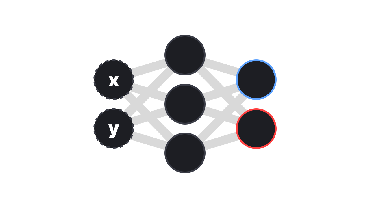
To design this network, we first need to determine what inputs it should receive. Since we’re classifying points on a 2D graph, we need two input neurons to represent the x and y coordinates of each point.

The network then needs to process this information through one or more hidden layers. For our problem, one hidden layer with three neurons turns out to be sufficient. This particular design choice is somewhat arbitrary. Determining the optimal number and size of hidden layers is more art than science, often requiring experimentation.

Finally, we need output neurons to tell us the classification result. Since we have two possible outputs (red or blue), we’ll use two output neurons. You might wonder why we don’t just use a single output neuron, with 0 representing red and 1 representing blue. There are two good reasons:

1. Using separate output neurons generalizes better to problems with more than two categories. For digit recognition, for example, we’ll use 10 output neurons (one for each digit) rather than encoding the digits in binary.
2. More importantly, giving each category its own neuron produces better results in practice. Each output neuron can focus exclusively on identifying the features specific to its assigned category.

The resulting neural network looks like this:

Implementing a Neural Network

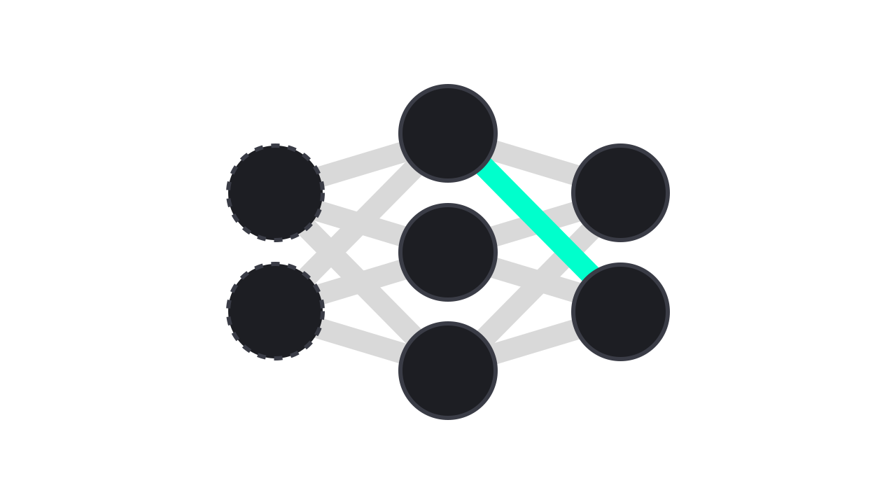
Before we can meaningfully see how to implement a neural network, we need to discuss the notation behind them. We’ll use $w^l_{jk}$ to represent the connections between the $k^{th}$ neuron in the $(l-1)^{th}$ layer and the $j^{th}$ neuron in the $l^{th}$ layer. The weight highlighted below would be written as $w^3_{21}$.

The ordering of the subscripts might seem strange, but this is so that the notation matches our other variables. We use $a^l_j$ to represent the activation of the $j^{th}$ neuron in the $l^{th}$ layer. The same notation is used for the biases, $b^l_j$, and weighted sums, $z^l_j$. Lastly, $f$ is our activation function. Using this notation allows us to relate the activation of a single neuron in layer $l$ to the neurons in the previous layer.

We can significantly clean this expression up by rewriting it in a way that focuses on the layers of the neural network. We can create a weight matrix $w^l$ whose entries are described by $w^l_{jk}$ where $j$ is the index of the row and $k$ is the index of the column. Similarly, the bias, weighted sum, and activations can be written as vectors $b^l$, $z^l$, and $a^l$, respectively.

To apply the activation function, we also need to discuss vectorization. Vectorizing a function means that we’re performing the element-wise application of a function onto the components of a vector (NumPy does this via broadcasting). Suppose we had the function $f(x) = x^2$. Then vectorizing $f$ has the effect of squaring each component of a vector passed to it.

This allows us to rewrite our original expressions using vectors and matrices, so that we can represent what’s going on layer by layer. This makes the equations much easier to understand while also giving a speed boost since many libraries optimize matrix computations.

Because the activations at each layer, $a^l$, depend on the activations of the previous layer, $a^{l-1}$, this forms a recursive structure. This means that each layer is applying a transformation to the output of the previous layer. Viewing a neural network as a deeply nested composition of functions is a useful perspective that will come in handy.

We can generate a prediction by feeding an input into the neural network—denoted as $a^1$—and then, using the recursive definition, computing the activations of the following layers until we reach the output, $a^L$. $L$ is the total number of layers.

Using Our Neural Network

We have no way of knowing if this network can actually accurately classify these points without testing it. We’re going to do that in the widget below. In it, you can adjust the weights and biases manually in order to get the network to correctly classify the points.

Don’t worry about being methodical. You don’t have to get all of them classified correctly, but playing around with it for a bit should give you a better feel for how the network functions. The top slider is the biases for each neuron, and the rest are weights.

While adjusting the sliders for the weights and biases, you likely ran into issues such as the decision boundary abruptly shifting at times. Ideally, what we’d want is a system where small changes in the weights and biases would cause small changes in the output of the neural network.

Michael Nielsen, in his book “Neural Networks and Deep Learning,” puts it perfectly:

If it were true that a small change in a weight (or bias) causes only a small change in output, then we could use this fact to modify the weights and biases to get our network to behave more in the manner we want. For example, suppose the network was mistakenly classifying an image as an “8” when it should be a “9”. We could figure out how to make a small change in the weights and biases so the network gets a little closer to classifying the image as a “9”. And then we’d repeat this, changing the weights and biases over and over to produce better and better output. The network would be learning.

However, this isn’t the case with the Perceptron. Perceptrons can only ever be 0 (off) or 1 (on). That means that adjusting their weights or biases can result in their output flipping. This flip can cause a cascading effect that causes other Perceptrons’ values to flip in some erratic way. This problem is already apparent in our tiny neural network, and it only gets worse as networks get larger.

Sigmoid Neurons

To solve this problem, we’re going to introduce a different type of neuron called the Sigmoid Neuron. Just like the Perceptron, it calculates a weighted sum and passes it to an activation function. Instead of returning 0 or 1, the Sigmoid Neuron returns a value between 0 and 1. Its activation function is called the sigmoid, and it can be written as follows:

If you’re wondering why this function was chosen, the reason is somewhat arbitrary. It’s mostly because the sigmoid is reminiscent of a smoothed-out step function. This makes it behave similarly to the Perceptron. Although it can’t take on the values 0 or 1, it can get extremely close given a large enough negative or positive value, respectively. In theory, you could create similar neural networks with either Perceptrons or Sigmoid Neurons. Sigmoid Neurons just happen to have much nicer properties to work with.

So how can we interpret the output of a Sigmoid Neuron? This is context-dependent and can change based on what you want the neural network to do. Oftentimes, it can be seen as a confidence score. If the output neurons corresponding to the red and blue labels are 0.97 and 0.3, respectively, then the neural network much more strongly believes that the point is red rather than blue, so we would classify the point as red.

If you’re hesitant about the fact that the sigmoid can never be 0 or 1, keep in mind that real-world data is noisy, so absolute certainty is unrealistic. If you’re still hesitant, my response to you is: can you ever be truly certain of anything? (‘I think, therefore I am’ is not a valid answer.)

The sigmoid itself isn’t special. In “Optimizing Training from Scratch” (a future course), we’ll explore other activation functions as we try to squeeze every ounce of performance out of our neural networks. For now, let’s revisit the tuning exercise from before, this time using the sigmoid, and see whether it’s gotten any easier now that we have a smooth and continuous activation function.

Tuning this neural network was probably much more intuitive than with Perceptrons. You still might have experienced some issues with large shifts. Those are just a consequence of using toggles. With more fine-grained controls, you would see that the shifts are smooth.

You might have observed some interesting phenomena, such as holes appearing out of nowhere. This isn’t a flaw. Neural networks are meant to be flexible, so that they can model complex behavior. Although this flexibility does cause issues at times, it’s generally beneficial, and there are ways of managing it.

Along with this growth, it becomes exponentially harder to manually tune a neural network. Modern networks like ChatGPT can have trillions of parameters. This highlights a crucial question: How can we systematically find the optimal weights and biases without guessing?

Looking Forward

In the upcoming lab, you’re going to get a chance to design a neural network that can classify digits. It won’t be much better than random because the parameters won’t be tuned, and it’s not feasible to manually tune the weights and biases due to there being thousands. In the following chapters, we’ll learn how to systematically update the weights and biases of a neural network by addressing what it means for a neural network to ‘learn.’