Chapter 2: Training Neural Networks

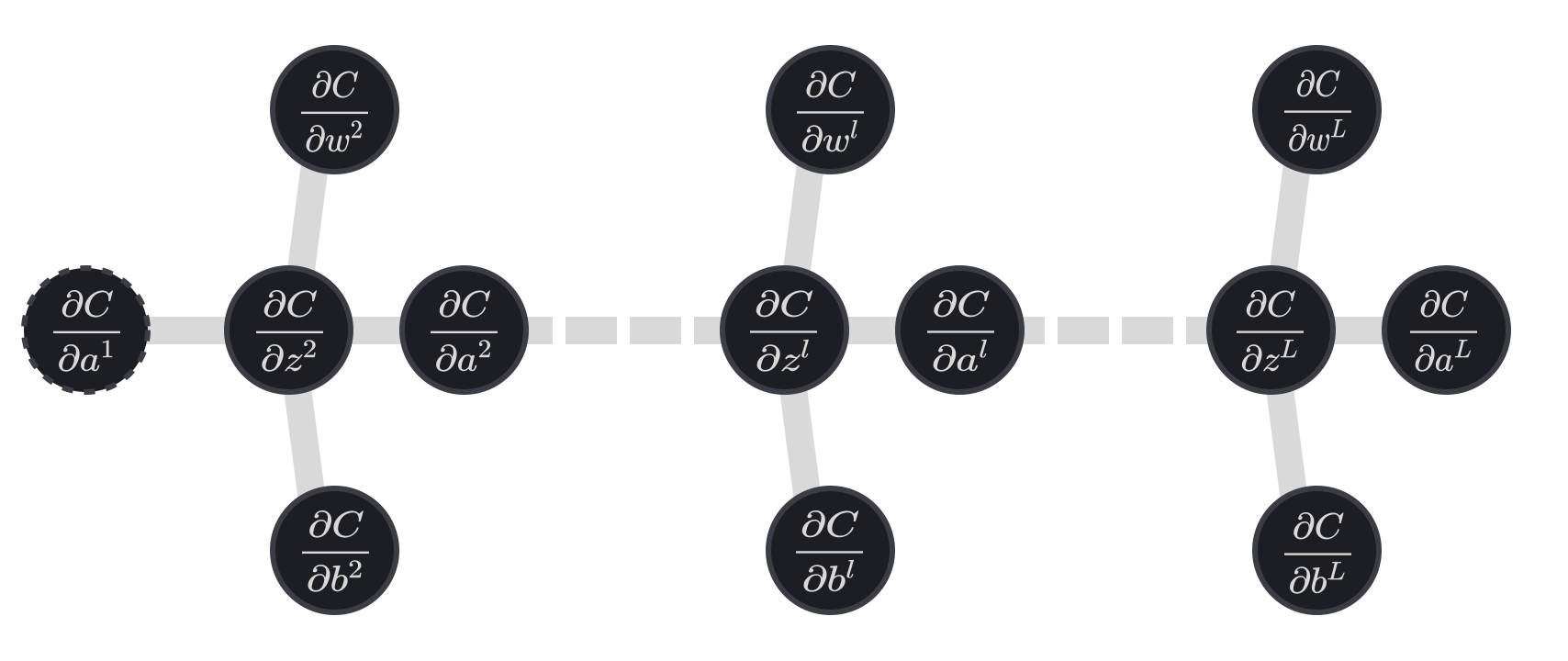
In the previous chapter, we explored the basic structure of a neural network and tried manually tuning a small one to classify points on a graph as either red or blue. It was a tedious process that was doable for our small neural network but got exponentially harder larger ones. To solve this problem, we need to find a way of getting neural networks to learn on their own.

What Does It Mean For A Model To Learn?

Before we can devise a method of getting neural networks to learn, we need a way of measuring their performance. A simple approach would be to feed the network a bunch of examples and count how many it gets right. However, we want to also know how close the network is to the answer so that we can reward the model as it gets closer to it.

Let’s revisit our point classification task. Remember that we represent the label for a blue point as the vector $y_{blue} = [1, 0]^T$ and a red point as $y_{red} = [0, 1]^T$ (assuming the first output neuron corresponds to blue and the second to red). Now suppose that we had two neural networks that classify points. We can feed them the same input point, $x$, that we know is blue, and the networks then produce the following predictions:

In this scenario, both networks incorrectly classify the point as red (since the red component’s activation is higher in both predictions). Based purely on accuracy, they both failed equally on this example.

However, intuitively $\hat y_2$ seems less wrong than $\hat y_1$. $\hat y_1$ is much more confident in its answer despite being wrong. $\hat y_2$ is much more uncertain about its decision. We can quantify this by looking at the distance between the prediction and the true label:

This kind of measurement lets us give partial credit to models that make predictions close to the correct answer—even if they’re technically wrong. It also encourages models to be more confident when they are right, since smaller distances to the true label reflect both correctness and certainty.

Cost Functions

We can rigorously define this using the cost function:

Here, $w$ represents the network’s weights, and $b$ represents the network’s biases. $n$ is the number of samples we train on. $y_i$ is the i-th label, and $\hat y_i$ is the neural network’s prediction using the i-th input. Although not explicitly written, $\hat y_i$ is dependent on $w$ and $b$.

This cost function is known as the Mean Squared Error, or MSE for short. While other cost functions exist, MSE is an excellent starting point for understanding how neural networks measure performance and begin the learning process.

Looking at the MSE, you should see that it’s non-negative because we square the error of every prediction before summing them up. Also, note that the worse the neural network’s predictions are, the larger the MSE gets. The inverse is also true: the better the neural network’s predictions are, the lower the MSE is. So the question of how we teach a neural network is the same as asking how to minimize the cost.

How Does a Neural Network Learn?

If you’ve taken a Calculus course (which you probably have if you’re reading this), your first instinct for minimizing a function should be to find where its derivative—or gradient—is zero. While this might work for tiny neural networks with a couple of parameters, analytical solutions quickly become unfeasible as networks get larger for a host of reasons. We won’t get too much into them, because they don’t give us much insight into the problem.

But to give you an idea, our tiny point classifier has 17 parameters, and our digit classifier has 12,175. Solving for the minimum analytically in these high-dimensional spaces is tedious and often impossible. This problem is made worse when you factor in how tightly coupled the parameters are and how deeply nested the functions become in deeper networks. So we need to find a different strategy that can scale well to higher dimensions.

Gradient Descent

For what we’re about to discuss, it would help to imagine a graph in 17 or 12,175 dimensions. Unfortunately, we’re limited to at most three, but if you could visualize the cost function for either of our networks, $C(w, b)$, you’d see a landscape filled with countless hills and valleys. A network’s weights and biases define a point on this landscape, and the height of that point corresponds to its cost.

We want an algorithm that finds the lowest point on this graph as quickly as possible. A helpful thought experiment is to imagine yourself lost at the top of a mountain and needing to find your way down. If you’re unable to see the bottom, you’d most likely choose to step in the steepest downward direction. Following this idea leads us to a powerful algorithm known as gradient descent:

In order to make use of our idea, we need to describe it mathematically. To keep the math from getting too out of control, we’re going to ignore neural networks for a bit. We can illustrate this approach well using a function of two parameters, $C(v_1, v_2)$. Keep in mind that this method easily extends to functions of much higher dimensions.

Our goal is to minimize the cost, so we can use Calculus to see how changing $v_1$ and $v_2$ affects the cost.

We can rewrite the equation as the dot product between the gradient and the direction we move in:

What we want to find is the direction, $\Delta v$, that causes the greatest decrease to the cost. You should remember from multivariable calculus that the gradient points in the direction of steepest ascent. So it should make sense that moving in the direction opposite to the gradient would give us the direction of steepest descent. We can write this as:

Here $\eta$ is a positive scalar known as the learning rate. It defines the size of the step we’re taking as we travel down the mountain. Plugging our equation for $\Delta v$ into our previous equation for $\Delta C$ yields us the following:

Because $\eta > 0$ and $\| \nabla C \|^2 \ge 0$, we can be certain that $\Delta C \le 0$. This guarantees us that moving opposite the gradient will cause the cost to decrease. So, what we want to do now is find the gradient and update $v$.

By repeatedly applying the update rule—finding the gradient and adjusting v—we should eventually arrive at a minimum. This is assuming that you’ve chosen a learning rate, $\eta$, that’s small enough to make for a good approximation while not being so small that it causes gradient descent to run unnecessarily slowly.

Applying gradient descent to neural networks is similar. The weights, $w_i$, and biases, $b_j$, define the point we’re at in our cost function. The gradient contains partial derivatives corresponding to each weight and bias in the network. We can use this information to define our update rules:

By taking small steps in the opposite direction of the gradient, you will eventually approach a minimum. Although this minimum may not be the global minimum, in practice, it still works phenomenally, as you can see in the widget below. The slider is used to adjust the learning rate of the neural network.

Hopefully, you played around with the widget long enough to notice two key things.

First, the neural network doesn’t usually classify every point correctly. This is normal. Neural networks aren’t always accurate, and we can fall into some local minima that aren’t great. You may have noticed this neural network sometimes settles on a poor linear boundary to classify the points. This problem is more apparent with small neural networks. In fact, research has shown that in very large networks, most local minima tend to be quite good—close in performance to the global minimum. These larger networks have more flexibility to model complicated patterns in data and can more easily “escape” poor regions of the cost landscape.

Second, if the learning rate is too high, the neural network will eventually start jumping around. You need to find a good balance between keeping the learning rate small enough that the network can learn but not so low that it learns unnecessarily slowly. The learning rate is often adjusted throughout the training process in order to maintain a balance between the two. In the next lab, you’ll implement the digit classifier using a constant learning rate.

Backpropagation

Throughout our discussion of gradient descent, I’ve purposely avoided explaining how to compute the gradient. Your first instinct is probably to manually differentiate to find the gradient, but that approach doesn’t work well with neural networks.

Finding the gradient of a cost function, $\nabla C$, involves finding the gradient of every single training example and then averaging them. We can derive this as follows:

The overall cost, $C$, is equal to the average cost of all individual training examples, $C_i$. Its form depends on the cost function used. For MSE, it’s written as:

Finding the gradient of the cost gives us:

Since gradients need to be computed for every training example and for every step we take during gradient descent, we need a way of efficiently computing the gradient. To solve this problem, we can use an algorithm known as backpropagation.

If you’re curious why naive approaches like numerical and symbolic differentiation don’t scale to networks with thousands or millions of parameters, our next course, Backpropagation from Scratch, covers that in depth. Here, we’ll focus on deriving the equations specific to neural networks.

Deriving the Four Fundamental Backpropagation Equations

The key insight into backpropagation comes from recognizing that each layer in a neural network is a function composition. Each layer depends on the layer before it, and ultimately, the cost function depends on the output of the final layer. This nested structure forms a chain of dependencies that can be exploited using the chain rule.

To compute the gradient for a training sample with respect to every weight and bias in a network, we start from the output layer and work our way backward. This is done using an intermediate value known as the error.

We will be denoting $C_i$ as $C$ for notational convenience in this section. The error, $\delta^l_j$, serves as a measure of how sensitive the cost is to a change in the $j^{th}$ neuron of the $l^{th}$ layer. You might wonder why the error is defined using the weighted sum rather than the activations, and the reason simply is because the equations for the backpropagation algorithm turn out simpler with it.

Finding the Error for the Output Layer

The point of backpropagation is to get closer to the desired output, and to do that, we need to start by addressing the error in the output layer, $L$. This leads us to the first of our fundamental equations:

The error of any given neuron in the output layer is equal to how much changing its output would affect the cost times how much the neuron’s output would change if we nudged its input. The form of $\partial C / \partial a^L_j$ depends on the cost function used. Since we used MSE, it’ll be equal to:

So far, we’ve written the output error in its component form. However, we prefer a matrix form because libraries optimize for them (resulting in a free speed boost), and it’s more intuitive to think of backpropagation and neural networks in terms of layers.

To do this, we need to introduce a lesser-known vector operation known as the Hadamard Product (or Schur Product). It’s denoted as $A \odot B$ and represents the elementwise product of two matrices that are the same size.

Using the Hadamard product, we can rewrite the error for the output layer as:

Here, $\nabla_a C$ is referred to as the gradient with respect to the output layer (the subscript $a$ may sometimes be written as $a^L$ to remove ambiguity). When using MSE, $\nabla_a C$ is equal to $a^L - y$, and its components are the partial derivatives $\partial C / \partial a^L_j$.

We’ll continue using the gradient notation instead in order to keep it more general.

Propagating the Error Backwards

It should stand to reason that the error in the output layer is, in part, caused by errors in the preceding layer. This relationship is described by the second fundamental equation of backpropagation.

Here, $(w^{l+1})^T$ moves the error back a layer, $l$. Then, taking the Hadamard product with $\sigma'(z^l)$ moves it past the activation function to get us the error, $\delta^l$. This equation in combination with the first allows us to compute the error for every layer in the network, starting with the output layer.

Adjusting the Weights and Biases to Minimize the Error

Now that we know how to find the error for any layer in the neural network, we need a way of using it to tell us how to adjust the weights and biases to decrease the error. We’ll start with the biases since they’re simpler to update. Because the bias doesn’t depend on any other parameter, we can directly adjust it to account for the error in the layer.

Weights are a bit more complicated. Since they’re reliant on the activation of the input neuron, we need to adjust the error by the activation of the input neuron.

We can rewrite this using matrices.

Implementing Backpropagation

Once you understand the equations for backpropagation, the algorithm should be relatively easy to understand.

1. Input: We pass the input to the network by setting the input layer, $a^1$.
2. Feedforward: After receiving the input, we feed forward through the layers, storing all the weighted sums and activations that we compute along the way. These will be used when we start backpropagating the errors.
3. Compute Output Error: Once we get the network’s results, we compare it to the label and find the output error.
4. Backpropagate Error: Using the output error, we compute the error for all of the previous layers. Along the way, we can compute the partial derivative of the weights and biases.
5. Output: At the end, backpropagation returns to us the gradient for the training example.

There are two interesting things to note about the algorithm. First, it’s typically appreciated through the lens of the chain rule. As we propagate the error backward and compute each partial derivative, we are effectively applying the chain rule.

However, the real efficiency comes from storing the values we get from the forward pass and the error term. This allows us to avoid unnecessary computations that approaches such as symbolic differentiation suffer from. If you’ve studied data structures and algorithms, you might recognize this as dynamic programming.

Stochastic Gradient Descent

Backpropagation only fixes the computational cost of calculating the gradient for a single training sample. Even with backpropagation, finding the gradient of the cost function, $\nabla C$, is still computationally expensive. It requires us to find the gradient for each individual sample of data, and then average it.

As the number of samples we have increases, learning slows down. Stochastic gradient descent can be used to speed this up drastically. Instead of averaging over every single data point, we create mini-batches, $X_1, X_2, ..., X_N$, whose sample size is $m$, that we use to approximate the gradient. The larger the sample size, the better this approximation gets.

The key idea is that we use this approximation to update the network’s weights and biases much more frequently. Instead of one update after processing the entire dataset (an epoch), we make an update after each mini-batch. So, for a dataset with $n$ samples and a mini-batch size of $m$, we perform $n/m$ updates per epoch. This allows the network to learn much faster, as it gets feedback more often.

Our update rules can now be rewritten as:

SGD should be intuitive. Getting the opinion of 100 people on a topic should give you a good idea of what the general population’s opinion is on that topic (given that you chose an unbiased sample).

There will be some statistical fluctuations in the gradient with SGD, but we just need to go in the general direction that decreases the cost, even if it’s not perfect. Doing this gives us a massive speed-up. In the point classifier, we have almost 1000 points we are trying to classify. Using a sample size of 30 allows learning to be ~33 times faster.

Escaping Local Minima and Saddle Points

We’ve seen that gradient descent can settle into mediocre local minima and get stuck. It turns out, SGD’s statistical fluctuations are useful here. Since each mini-batch, $X_j$, only approximates the gradient, it’s unlikely to be exactly zero even at a point where the actual gradient is. This noise can be enough to knock the network out of a shallow local minimums.

This noise matters even more for saddle points. These are points where the gradient vanishes but the surface still curves upward or downward in some directions. Gradient descent can sometimes get stuck in these saddle points, but the noisy nature stochastic gradient descent allows it to escape these points and keep learning.

Looking Forward

You’re now going to take the neural network you designed in the previous lab and implement stochastic gradient descent along with backpropagation to teach it to classify digits. After implementing your neural network, we’ll take a deep dive into what’s actually going on behind the scenes. So far, we’ve taken a technical view into training a neural network, but it’s beneficial to take a step back and get a more intuitive understanding of the algorithms.