Chapter 3: Behind the Scenes of Training

In the last chapter, we took an analytical approach to training a neural network, but it’s helpful to take a step back and understand what’s going on and what the math is actually telling us.

What’s Backpropagation Actually Doing?

Backpropagation tends to be seen as a bit of a monster when it comes to understanding neural networks, but it turns out to be an intuitive method of updating the weights of the neural network. If you were to look at an untrained neural network’s prediction for a given input and then compare it to the label, what you’d find is that there’s a mismatch.

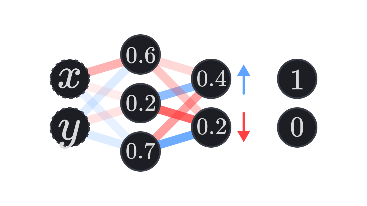
Ideally, we want the prediction to match the label. To do this, we need to adjust the output of the neural network to more accurately match the desired label. This means increasing the output of the neurons that should fire and decreasing the ones that shouldn’t. We have three ways of adjusting a neuron’s output.

The Bias

The bias is the most straightforward way of adjusting a neuron since it doesn’t rely on or affect anything besides the neuron it corresponds to. If a neuron is supposed to be more active, we increase its bias. If it’s too active, we decrease it. How much we adjust it depends on how far off the neuron is from the desired activation.

Adjusting the Weights

Adjusting weights is a bit more involved, since their effect depends on the activations coming from the previous layer.

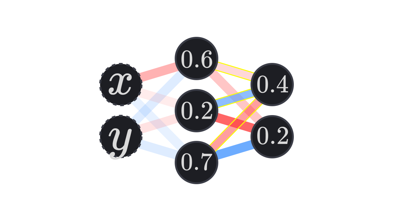
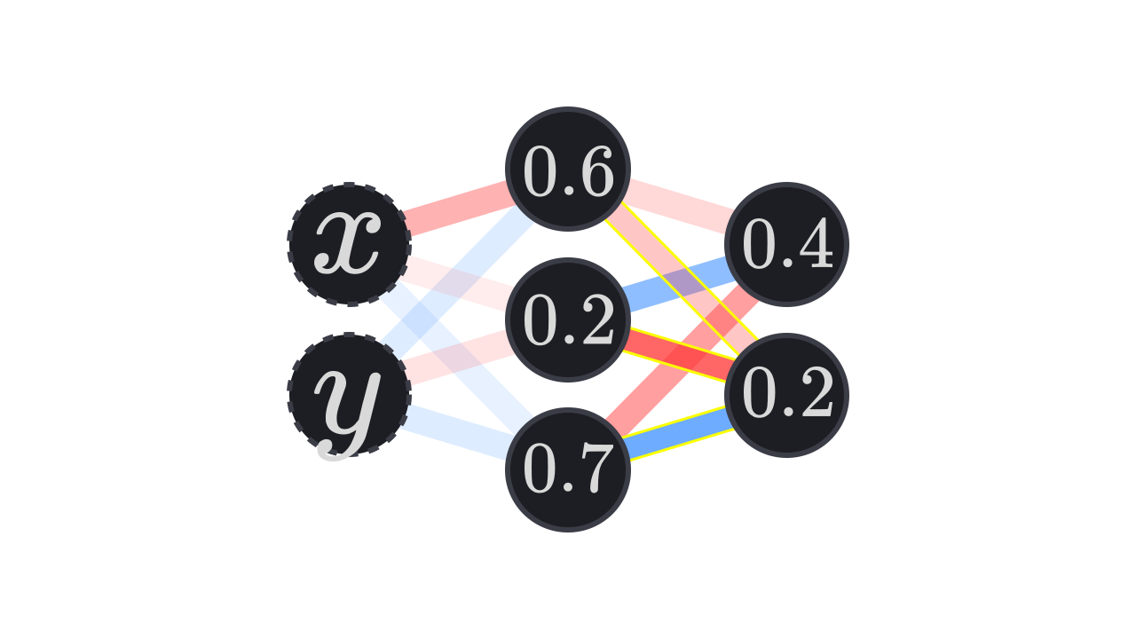
We can increase the activation of underactive neurons by increasing the value of the weights activating it and dimming the weights driving it down. Inversely, for overactive neurons, we can dim the weights activating it and strengthen the weights deactivating it to drive its activation value down.

To increase the activation of 0.4, we want to decrease the negative weights and increase the positive weight.

To decrease the activation of 0.2, we want to increase the negative weights and decrease the positive weight.

Not every neuron in the previous layer gets an equal say. The neurons that actually fired for this input are the ones driving the current layer’s output. So a weight attached to a highly active neuron influences the result much more than one attached to a neuron that barely activated. So when the output is wrong, the weights connected to those active neurons carry most of the responsibility, and they’re the ones we adjust the most. Weights from quiet neurons hardly affected the decision, so they’re left mostly untouched.

The process of adjusting each weight proportionally to how much its input neuron “participated” causes connections with highly active neurons to get reinforced (or weakened) more strongly. In effect, neurons that activate together during training tend to strengthen their connection over time. In other words, neurons that fire together, wire together.

This principle is borrowed from neuroscience and explains how neural networks learn patterns. When certain combinations of features consistently appear together in the training data, the weights connecting those features become stronger, making the network more likely to recognize similar patterns in the future.

Adjusting the Previous Layer’s Activations

So far, we’ve seen how to adjust a neuron’s bias and weights to improve the output. But the error in a neural network isn’t caused by one layer alone. In order to update the weights and biases properly, we need to know how each neuron in the previous layer contributed to the error.

Every neuron in the current layer has an opinion on what the previous layer should do. Neurons whose output needs to be increased want to increase the activations of neurons associated with positive weights and decrease those associated with negative weights.

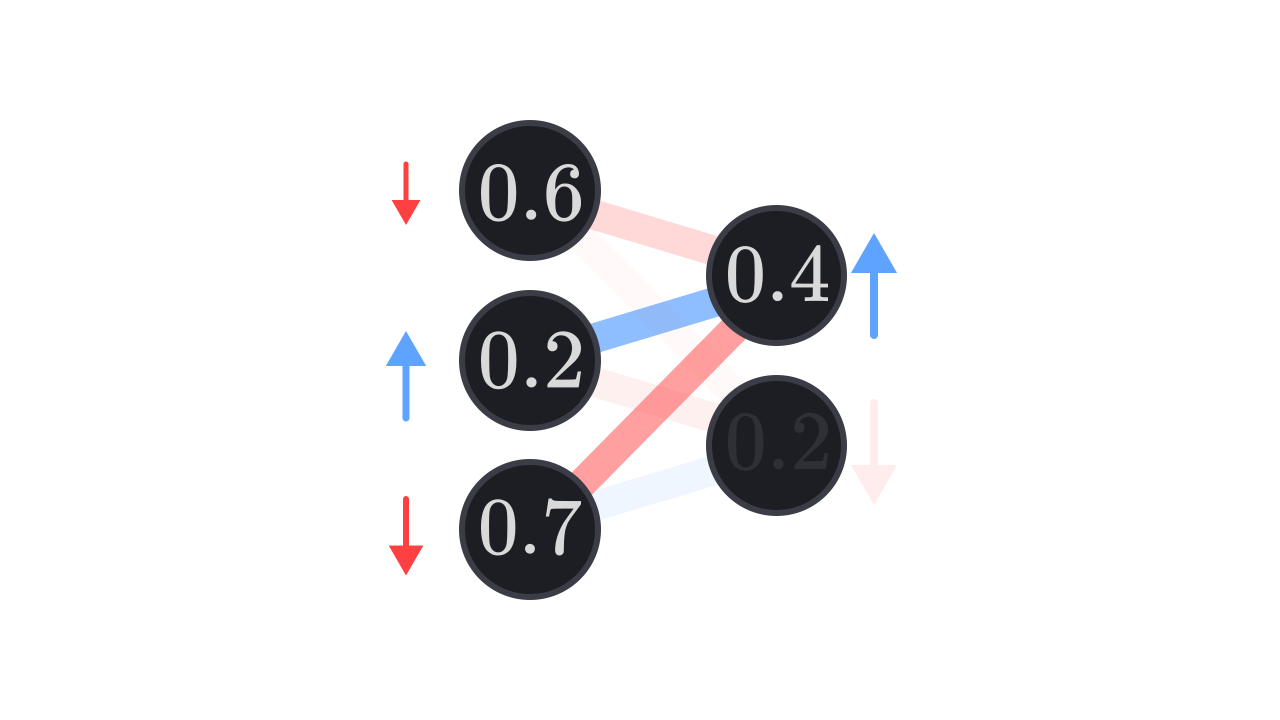
The size of an adjustment is proportional to the weight because it determines how strongly an activation influences the next layer’s neurons, so a larger weight means that an activation is more responsible for the next layer’s error and needs a correspondingly larger adjustment to correct for it.

To reduce a neuron’s output, we do the opposite. We increase the activations coming through negative weights and decrease those coming through positive weights.

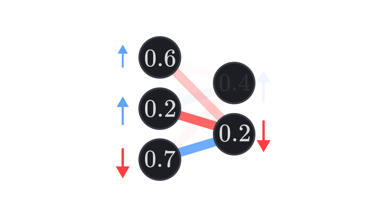
Since every neuron has a slightly different opinion on how each neuron should change, we combine them to figure out the ideal adjustment.

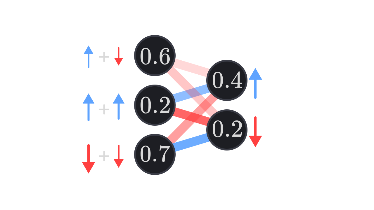
This process of passing the blame backward is called backpropagating the error, and it is described by the following equation.

Random Initialization

When backpropagation is updating a neuron’s weights and bias, it doesn’t consider what other neurons in the same layer are doing. If every parameter starts with the same value, every neuron in the layer is going to behave identically. This means they’ll receive the same updates since their gradients are identical, and they’ll end up learning the same features. Effectively, you end up with one neuron per layer.

To break this symmetry, we initialize the weights and biases with random values. These are typically sampled from a standard normal distribution. This ensures that each neuron starts off a little different, allowing them to specialize in different ways as training progresses.

There’s another reason random initialization matters: if all the weights and biases are set to zero, the network might not learn at all. Zero inputs lead to zero outputs, which can cause zero gradients, depending on the activation function.

What’s Gradient Descent Actually Doing?

When backpropagation processes a single training example, it computes adjustments that would make the network perform perfectly on just that one case. For instance, if we show the network a poorly written “3” that looks somewhat like an “8”, backpropagation might suggest changes that help distinguish that particular “3” from an “8”. But these changes might actually hurt the network’s ability to recognize clearer examples of “3”s or “8”s.

The process of finding gradients and averaging over all of them coerces the neural network to learn more general patterns in the data in order to make better predictions. This process is one way of protecting against overfitting. Overfitting is the tendency for networks to memorize training examples rather than learn generalizable patterns.

However, we use a variation of gradient descent known as stochastic gradient descent, which introduces controlled randomness in an effort to keep computational cost low. It turns out that the randomness actually helps the network find better solutions. It helps the network escape saddle points more efficiently and generalize better. Because the gradient is constantly changing due to the randomness in the mini-batches, the network is discouraged from overfitting and becomes more robust against noise.

Looking Forward

We’ve learned how to design and train a neural network from scratch. You now understand the fundamental concepts behind neural networks, from their basic structure to how they learn through backpropagation and gradient descent. While many techniques and optimizations exist beyond what we’ve covered, you have a solid foundation to build upon.

In the next chapter, we’re going to briefly discuss how you can go about interpreting what a neural network is actually learning, and how you it learns to classify digits.